The Constant Caterer

At my place of work they’ve got taste. While the building’s exterior looks like you’d expect after 30 minutes by train and ten minutes by foot from the center of Paris, on the inside it looks like an interior decorator went to town and came back with a wheelbarrow’s worth of vases, books, and poofs. It’s sophisticated. In fact, when I first came there I recognized some of these gizmos because I considered getting them for our apartment after we moved in a few years ago.

Once, when trying to get from Aft to Bow through the office’s maze of corridors, phone booths, meeting rooms, and adjustable desks, this little number caught my eye:

Alt text: Photograph of a vase in the shape of the letter ‘h.’

‘How appropriate for a quantum computing company,’ I thought, ‘a vase in the shape of the Planck constant!’ Immediately chased by the feeling that, unless if you’re Maltese, it would certainly look more quantum if it had a horizontal stroke resembling the reduced Planck constant, $\hbar = h/2\pi$, instead. But would that actually make it more quantum?

I started pondering: how would I describe what the Planck constant represents? And which is the preferred one, $h$ or $\hbar$? At its face, this sounded like a sophomoronic dilemma along the lines of: ‘Is a tomato a fruit or a vegetable?’ Or: ‘Tea in first, or milk in first?’ Or: ‘Is a chair finely made tragic or comic?’[1] But the Planck constant pulls some pretty weird stuff, and I’d like to argue that this is a question worth asking. Allow me:

Exhibit A

The Planck constant comes at you in undergrad as a proportionality factor between the frequency of a photon ($\nu$) and its energy:

\[E = h \nu.\]

Its units are J/Hz, but thinking of it as “Nature’s proportionality factor that converts frequency into energy” doesn’t exactly cover it, as the other items that have been entered into evidence will show.

Exhibit B

We also encounter Planck’s constant in the Schrödinger equation, where it relates the rate of change of a system’s wave function $\psi$ to its Hamiltonian $\mathcal{H}$:

\[i\hbar \frac{\partial\psi}{\partial t} = \mathcal{H} \psi.\]

Here, $\hbar$ ‘converts’ the rate of change in $\psi$ (which has units s$^{-1}$) to energy, so in terms of dimensions it fulfills its bookkeeping duty, but surely $\partial \psi /\partial t$ is something more generic than a frequency.

Exhibit C

Things get progressively more disconnected from energy/frequency conversion as we consider Heisenberg’s uncertainty principle, where the connection seemingly goes out the window altogether. ‘Heisenberg’ states that the uncertainty in position and momentum ($\sigma_x$ and $\sigma_p$, respectively) are lower-bounded by: $\sigma_x \sigma_p \geq \hbar/2$.

Exhibit D

And what about angular momenta? We encounter spin and orbital angular momentum, for example, in multiples of $\hbar/2$ and $\hbar$, respectively. Angular momentum, here, is the quantum mechanical equivalent of $\vec{r} \times \vec{p}$, which carries the same unit as Heisenberg’s uncertainty relation quoted above. Granted, at least for orbital angular momentum one can argue it’s a consequence of $\vec{p}$ being defined in terms of $\hbar$, which can be retraced to how the Schrödinger equation is typically derived. (This has all the trappings of a circular argument, though.)

Why is it that, every time a quantity with dimensions ML$^2$T$^{-1}$ pops up, $h$/$\hbar$ is somehow involved? We’d be forgiven to think that the Planck constant is not unlike the character named Ice from Arrested Development, who in addition to his catering gigs doubles as a bounty hunter. These two professions seem orthogonal, but if you think about it, they both involve ensuring items are delivered from Alice to Bob in an orderly manner.

Is the Planck constant pulling a similar stunt? Can we find a metaphorical frame of reference from which all of $\hbar$’s jobs look more coherent, and which goes beyond the undergraduate’s adage: “If it’s got $\hbar$, it’s quantum!”

Ding dong, wave packet delivery!

Richard Feynman was a master of teaching: the skill of stringing along an audience into thinking complicated things are easy (the opposite of ‘bamboozling,’ in a way¹). Here, in this example from the Feynman Lecture on the principle of least action [2], he’s up to his usual spiel: in one paragraph he manages to explain the essence of quantum field theory while, in passing, shedding some light on the meaning of $\hbar$:

The complete quantum mechanics (for the nonrelativistic case and neglecting electron spin) works as follows: The probability that a particle starting at point 1 at the time $t_1$ will arrive at point 2 at the time $t_2$ is the square of a probability amplitude. The total amplitude can be written as the sum of the amplitudes for each possible path — for each way of arrival. For every $x(t)$ that we could have — for every possible imaginary trajectory — we have to calculate an amplitude. Then we add them all together. What do we take for the amplitude for each path? Our action integral tells us what the amplitude for a single path ought to be. The amplitude is proportional to some constant times $e^{iS/\hbar}$, where $S$ is the action for that path. That is, if we represent the phase of the amplitude by a complex number, the phase angle is $S/\hbar$. The action $S$ has dimensions of energy times time, and Planck’s constant $\hbar$ has the same dimensions. It is the constant that determines when quantum mechanics is important.

Note that here $S$ is the classical action: the integral of the difference of kinetic and potential energy taken over the particle’s path. In this reading, quantum mechanics more or less satisfies the principle of least action, but allows excursions on the order of $\hbar$ around the trajectory that minimizes $S$. Bundles of paths that deviate by significantly more than $\hbar$ from the optimum will have a rapidly varying phase factor among themselves, and will interfere destructively when they’re summed over. Put differently: $\hbar$ describes the fluctuations that quantum mechanics allows Nature to take in getting things from A to B.

How you can actually calculate something armed with this knowledge is a different question, and is generally within the purview of quantum field theory. The basic stage directions go something like this: using the path integral approach it’s possible to define a propagator that tells you the likelihood the system is taken from $|\psi_i\rangle$ at $t_1$ to $|\psi_j\rangle$ at $t_2$ (see e.g. the first chapter of Ref. [3] for a compact derivation). This is generally an integral over all possible paths, though, which isn’t easy to calculate (if it is at all calculable). Various approximations consist of identifying relevant selections of paths that can be summed over, while ignoring others, and which produce reasonable results [4]. Feynman invented a graphical language to describe and categorize different terms in the summation (his eponymous diagrams), and by ‘summing over’ various types of them the propagator can be approximated.

Moreover, as Feynman discovered when he was a graduate student, it’s possible to derive the Schrödinger equation from the path integral approach. (Disappointingly, I couldn’t find an account of this in the Feynman Lectures, but Ref. [5] does a good job — and, as a bonus, contains an entertaining account of how Feynman made the connection.)

What is interesting about this approach is that whole swaths of quantum mechanics can now be understood through arguments related to the action, which, via its ratio with $\hbar$ sets the phase of wave function components. The Planck constant, then, functions as a measuring stick that tells us whether changes in the action between a bundle of paths are small enough to require quantum mechanical attention. (The assumption being that the coherence will wash out very quickly if the fluctuations become large.)

From this principle it’s possible to (at least hand-wavingly) explain away 3½ of the four Exhibits outlined above: from the Schrödinger equation (and the momentum operator it implies) we can get Heisenberg’s uncertainty relation along with orbital angular momentum (of the $\vec{r} \times \vec{p}$ variety). Applying the Schrödinger equation to a two-level system with energy splitting $E$ exposed to radiation, we find that we get resonant transfer if we drive at frequency $\nu = E/h$ (doing this properly requires a few intermediate steps, though). Note that this reasoning doesn’t bother much with intrinsic angular momenta such as electron spin, but understanding this properly requires relativistic quantum mechanics which is very much for another time.

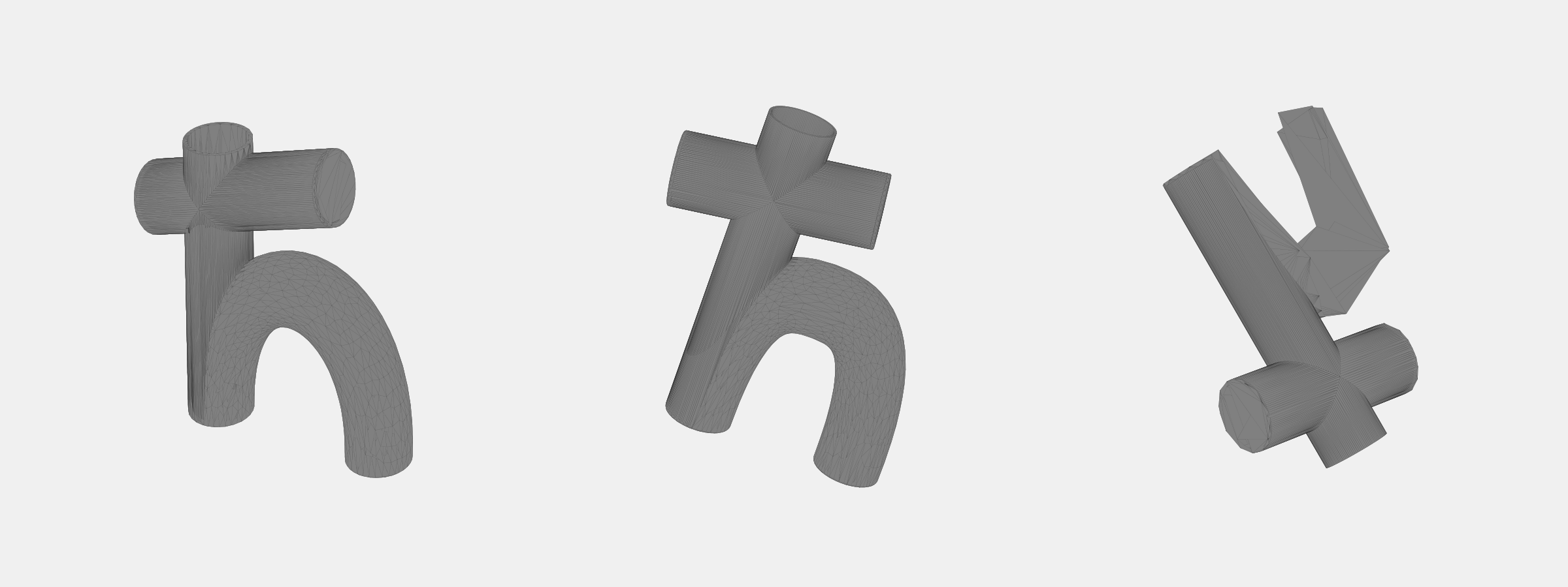
An improved horticultural receptacle

Having argued that $\hbar$ is the better Planck constant, I felt it was only appropriate to design an improved version of the little vase I encountered at work. So, in a moment of action I opened up the PartDesign workbench in FreeCAD, and — after a questionable number of botched fusions and failed connects — I managed to render it (with an angular momentum far exceeding the thing it refers to):

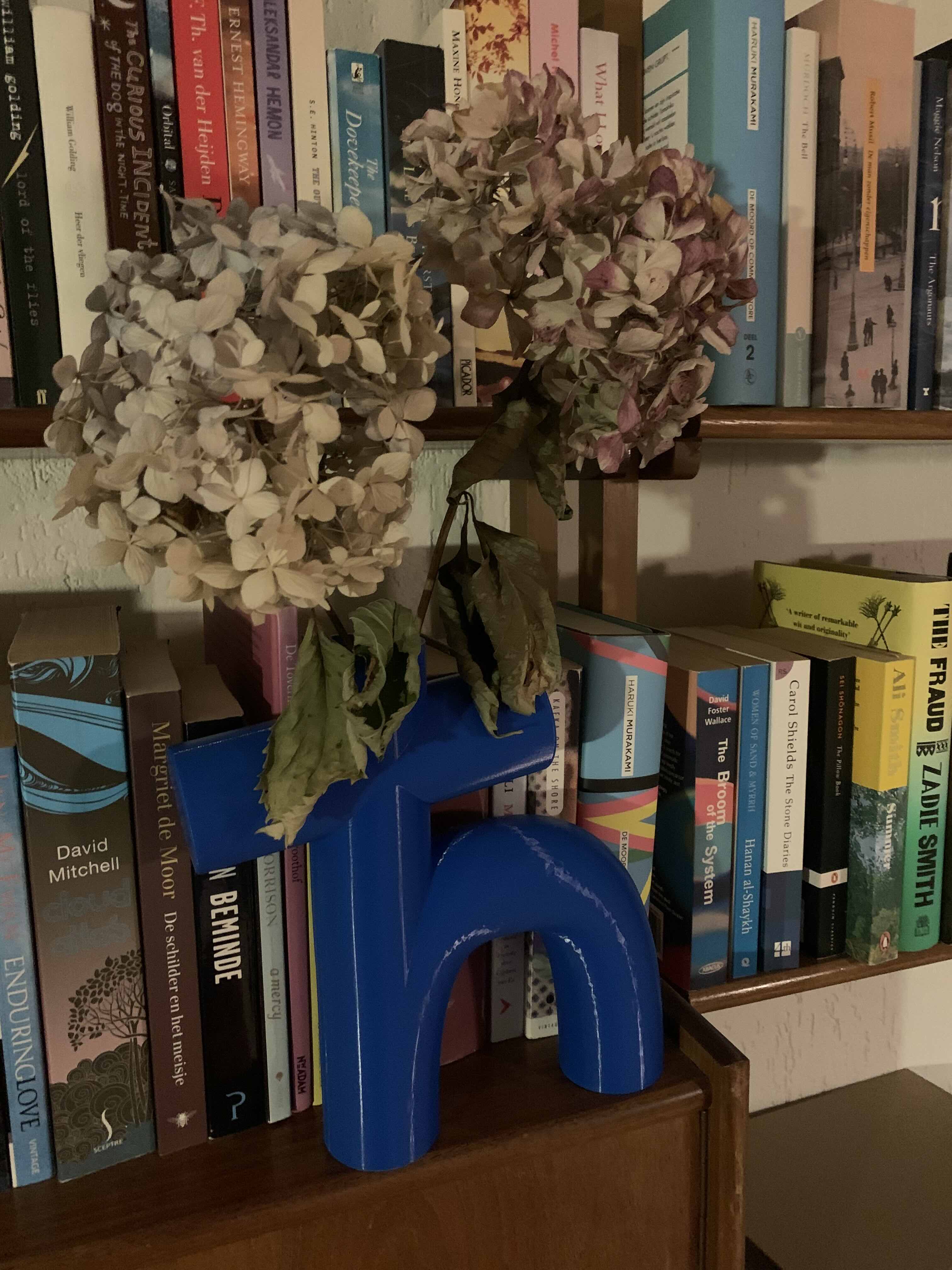
Nice, I thought, but wouldn’t it be better yet to render it in the office? So, in the spirit of the 2025 International Year of Quantum Science and Technology that is now drawing to a close, I combined quantum science with technology, and had the $\hbar$ vase 3D printed. Below shown in use as a container for some dried $\hbar$ydrangeas. (And, if you insist, you can find the .stl file here.)

References

[1] J. Joyce, A Portrait of the Artist as a Young Man, 1916.

[2] R.P. Feynman et al., The Feynman Lectures on Physics, Chapter 19: The Principle of Least Action, 2013.

[3] A. Zee, Quantum Field Theory in a Nutshell, Second Edition, Princeton University Press, 2010.

[4] R.D. Mattuck, A Guide to Feynman Diagrams in the Many-Body Problem, Second Edition, Dover Publications, 1976.

[5] D. Derbes, Feynman’s derivation of the Schrödinger Equation, American Journal of Physics, 64 (7), 1995.

Note

1. Bamboozle, verb [T]: to trick or deceive someone, often by confusing them. Cambridge English Dictionary. ↩